The timing of bad luck.
When one adverse outcome becomes hard to unlearn
A bad result can change what an agent samples next. This note isolates how the time of that result, the learning-rate rule, and the number of TD backups between outcome and choice determine whether the agent ends with the wrong policy.
THE QUESTION
Bad evidence changes future evidence.
A learner does not passively receive a fixed dataset. What it currently believes changes what it chooses, and therefore what it gets to observe next.
An adverse result on a promising route can make that route non-greedy. If exploration is already declining, the agent may then stop collecting the observations required to correct the estimate. The broad phenomenon is known as the hot-stove effect; it was described in adaptive learning well before this note. Denrell and March showed how bad samples can suppress the sampling that would undo an underestimate, and Shteingart, Neiman, and Loewenstein measured lasting first-outcome effects in human choice.
Question. Under a fixed training budget, when does one adverse terminal outcome have the greatest chance of changing the final greedy policy?
The existence of path dependence is not the claim. The narrower object here is its timing profile, and how that profile changes when the estimator carries prior evidence differently and the outcome is several TD backups away from the choice.
THE INTERVENTION
One choice, one controlled shock.
At the start, the agent chooses between two routes. The safe route terminates immediately for . The risky route enters a deterministic chain and ordinarily terminates for . Its depth counts the state-action values from the start decision through the terminal predecessor. There are no later choices, and . The risky route is therefore truly optimal at every depth.
Before an event at training round , I calibrate exactly successful risky traversals. The risky values equal one and their visit counts equal . I then force the risky route once. The treatment receives at the terminal transition; its paired control receives the ordinary reward one. Every later risky outcome is again one, and the two arms share the same future random numbers.
This is an impulse response, not a simulation that waits for a rare event to occur naturally. If the bad reward arose with probability in a stationary reward distribution, the risky route would still have the higher mean whenever . Here I condition on one event so its causal effect can be estimated without a giant rare-event sweep.
- Training horizon
- 200 route choices
- Exploration
- ε: 0.40 → 0.01
- Step sizes
- 1 / N and α = 0.20
- Paired samples
- 20,000 per point
The outcome is finite-budget policy error: the probability that the treated learner finishes safe-greedy while its paired ordinary-outcome control remains risky-greedy. “Lock-in” below always means this operational, finite-horizon event.
THE EXACT CASE
At depth one, recovery can be counted.
Suppose the adverse result follows ordinary risky outcomes and is followed by more. Under a sample-average update,
The number of later risky visits required to make that action greedy again is
For the displayed rewards this is . Accumulated evidence eventually makes one late loss too small to reverse the ranking.
With a constant step size, the event instead moves the estimate to
and after later ordinary outcomes,
At , recovery always requires 12 risky visits, regardless of how much evidence preceded the event.
While risky is non-greedy, its possible recovery visits over the remaining horizon are
Because epsilon changes with time, is Poisson-binomial. For update rule , the exact depth-one error probability is
The recovery counts are equal after 48 prior successes. Before that point, sample averaging is more vulnerable; afterward, constant alpha is more vulnerable. The ordering follows from the recovery thresholds and does not depend on the particular epsilon schedule. The probability levels do.
EXACT DEPTH-ONE CALCULATION · b = −5
| Event round | Sample average | Constant α |
|---|---|---|
| 0 | 1.000 | 0.013 |
| 48 | 0.473 | 0.473 |
| 60 | 0.000 | 0.692 |
| 100 | 0.000 | 0.994 |
THE SECOND CLOCK
A terminal outcome must reach the choice.
One-step TD updates the risky chain online in forward order. In the adverse traversal, earlier links bootstrap from successors that have not yet received the bad target. Only the terminal predecessor changes immediately. Additional risky traversals are required for the shock to travel back to the start.
This creates two clocks. The first governs propagation of the loss to the start decision. The second governs propagation of later ordinary outcomes that repair the estimate. Once the start becomes safe-greedy, the route traversals needed for repair arrive primarily through declining exploration.
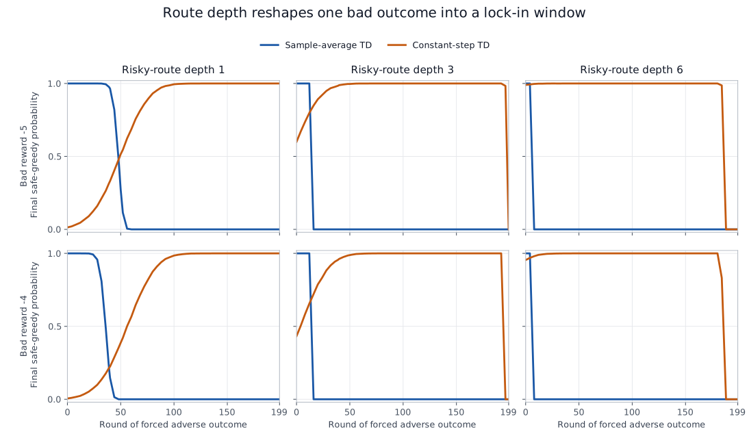
At event round 48, depth one is the analytic crossover: both rules finish safe-greedy in 47.8% of paired simulations. At depth three, the corresponding probabilities are 0.0% for sample averaging and 99.7% for constant alpha. At depth six they are 0.0% and 100.0%.
The nearby condition reproduces the separation. At its depth-one crossover, round 39, the two rules both finish safe-greedy in 21.4% of simulations. At depth three the probabilities are 0.0% and 95.6%; at depth six, 0.0% and 99.99%.
Depth also creates a late propagation blind spot. With constant alpha and depth six, an event at round 184 changes the final policy in 98.7% of runs. At round 188 it changes none: twelve remaining rounds are insufficient for the terminal target to reach the start. That zero is delayed credit, not recovery.
A full-return update sends the terminal outcome to every risky state in the same traversal. Its curve is therefore identical to depth one at every tested route depth. The change in Figure 1 comes from one-step temporal credit propagation, not from adding inert states to the diagram.
THE READING
Robustness and responsiveness are the same lever.
Sample averaging gives each new outcome less weight as evidence accumulates. That protects a mature estimate from a late isolated shock. Across several TD links, the attenuation compounds: after enough prior traversals, the terminal disturbance never pushes the start value below the safe value.
A constant step size preserves sensitivity to new outcomes. That is useful in a changing world, but here it preserves the size of the shock while the remaining exploration budget contracts. Route depth delays the policy change, then delays its repair even more.
This is not evidence that sample averages are generally better. Their immunity to late evidence is also an inability to adapt quickly. Nor is constant alpha intrinsically defective: the finite-horizon failure depends on an annealed behavior policy that stops revisiting the demoted route.
LIMITS
A controlled mechanism, not a general theory.
The safe value is known and fixed. The pre-event history contains a calibrated number of successful risky traversals rather than a naturally generated trajectory. Rewards and transitions are otherwise deterministic. The risky chain has no decisions after the start and uses discount one.
The results do not establish the same timing window for eligibility traces, replay, function approximation, recurrent agents, or deep RL. They also do not establish novelty. Early-outcome dependence and the hot-stove effect have an existing literature; deep RL has a separate, function-approximation form of primacy bias.
The contribution of this note is deliberately smaller: an exact depth-one impulse response and a paired demonstration that one-step backup depth creates a propagation-and-recovery window, including a late horizon blind spot.
REPRODUCIBILITY
One script and three compact artifacts.
The complete calculation and simulation run from one study-specific Python entry point. It does not use the laboratory's experiment protocol, a notebook, or raw Parquet shards. The published CSV contains every plotted estimate and confidence interval; the JSON file records the intervention, parameters, headline values, and deterministic propagation windows.
Results (CSV)Analysis record (JSON)Figure (SVG)
Open the analysis code